Building interpretable decision trees

In this post, we explore how to build Decision Trees so they are interpretable . Our goal will be to give the simplest model that retains the predictive power of a more involved model.

We will use the Titanic dataset for its simplicity in this workflow, however the method can be applied to many other datasets. You can find the complete script for this workflow here. The links within this post redirect to the Data-Archive, my second brain for all things data and modelling. The Archive acts as part of my research flywheel, more on that another day. Let us begin by looking at the data and building the Best model.

But First the Data

The Titanic dataset is used in a classic binary classification problem where the goal is to predict passenger survival (1 for survived, 0 for not survived). Before diving into the workflow process, we preprocess the data by:

• encoding categorical variables (e.g., converting “Sex” into numeric values), and
• imputing missing values (e.g., filling missing “Age” values with the mean).

After preprocessing, the dataset looks like this:

Pclass	Age	Fare	Sex_male	SibSp	Parch	Survived
3	22	7	1	1	0	0
1	38	71	0	1	0	1
3	26	8	0	0	0	1
1	35	53	0	1	0	1
3	35	8	1	0	0	0
…	…	…	…	…	…	…

Hyperparameter Tuning with Grid Search

To identify (our) Best Decision Tree configuration, we use GridSearchCV to systematically tune key hyperparameters such as:

• max_depth: which controls the maximum depth of the tree,
• min_samples_split: the minimum number of samples required to split a node,
• criterion (Gini, Entropy): the function to measure the quality of a split.

Here’s how we set up and run the grid search:

# Define the parameter grid
param_grid = {
    'max_depth': [2, 3, 5, 7, 10, None],
    'min_samples_split': [2, 5, 10],
    'min_samples_leaf': [1, 2, 4],
    'criterion': ['gini', 'entropy']}

# Perform grid search
grid_search = GridSearchCV(DecisionTreeClassifier(random_state=42), param_grid, cv=5, scoring='accuracy')
grid_search.fit(X_train, y_train)

Our Best model from the grid search uses the following hyperparameters:

Hyperparameter	Value
criterion	Gini
max_depth	3
min_samples_leaf	2
min_samples_split	2
random_state	42

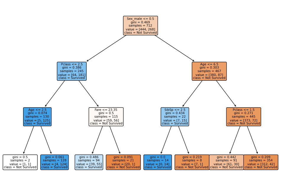
and has the following form:

Evaluating using 5 fold cross-validation, which we do in every case when determining Classification Metrics, gives an evaluation matrix of the form:

Metric	Mean	Std
Accuracy	0.8103	0.0121
Precision	0.7966	0.0185
Recall	0.6812	0.0559
F1 Score	0.7325	0.0302
ROC AUC	0.8499	0.0273

One could argue that such a tree is to large to be understandable. We will now reduce its complexity while retaining its predictive power (an approximate accuracy of 0.81).

Simplifying a Decision Tree

For Decision Trees the two most common methods to increase interpretability are to prune or do feature selection. Feature selection (FS) improves interpretability by reducing the number of variables in the model dataset. Whereas pruning trims unnecessary branches in the tree, simplifying its structure while maintaining performance. For Decision Trees it is important to determine whether FS should be done before or after pruning a model, as each has pros and cons.

FS before pruning:

• Reduces the input space early.
• Uses the full complexity of the model to determine feature importance.
• Helps mitigate overfitting.

FS after pruning:

• Aligns with a simplified model.
• Focuses on interpretability and prioritises simplicity over performance.

Since the Titanic dataset is relatively small, and we aim to maintain predictive power, we perform FS before pruning.

Base Model

We use Recursive Feature Elimination (RFE) to identify the most important features. RFE helps to iteratively remove the least important features. Here’s how we applied RFE:

from sklearn.feature_selection import RFE

# Apply RFE to the best model
rfe = RFE(estimator=best_model, n_features_to_select=3)
rfe.fit(X_train, y_train)

# Extract selected features
selected_features = [features[i] for i in range(len(features)) if rfe.support_[i]]
print("Selected Features:", selected_features)

The top three features are Pclass, Age, Sex_male. We will use this subset for subsequent modelling steps.

We can further simplify the model by increasing the size of the bins that values are partitioned into. Suppose we take the feature selected dataset and construct the Decision Tree model with the following Base hyperparameters.

Hyperparameter	Best Value	Base Value
criterion	Gini	Gini
max_depth	3	3
min_samples_leaf	2	10
min_samples_split	2	4
random_state	42	42

Recalculating the evaluation metrics for the Base model we obtain arguable similar results, while simplifying the model complexity.

Metric	Best Mean	Base Mean	Best Std	Base Std
Accuracy	0.8103	0.7963	0.0121	0.0213
Precision	0.7966	0.7902	0.0185	0.0931
Recall	0.6812	0.6493	0.0559	0.0837
F1 Score	0.7325	0.7036	0.0302	0.0387
ROC AUC	0.8499	0.8422	0.0273	0.0150

Pruning

Now that we have a simplified model and a reduced dataset, we can prune the model using cost-complexity pruning.

This method determines the optimal pruning threshold (ccp_alpha). We achieve this with the following snippet:

# Get the pruning path
ccp_path = base_interpretable_model.cost_complexity_pruning_path(X_train_rfe, y_train)
ccp_alphas = ccp_path.ccp_alphas

When we evaluate the Base model pruned using various ccp_alpha values using cross-validation for accuracy we get:

ID	ccp_alpha	accuracy
1	0.000000	0.796297
2	0.000412	0.796297
3	0.003874	0.794888
4	0.004331	0.796297
5	0.009055	0.786467
6	0.015924	0.783650
7	0.038605	0.778046

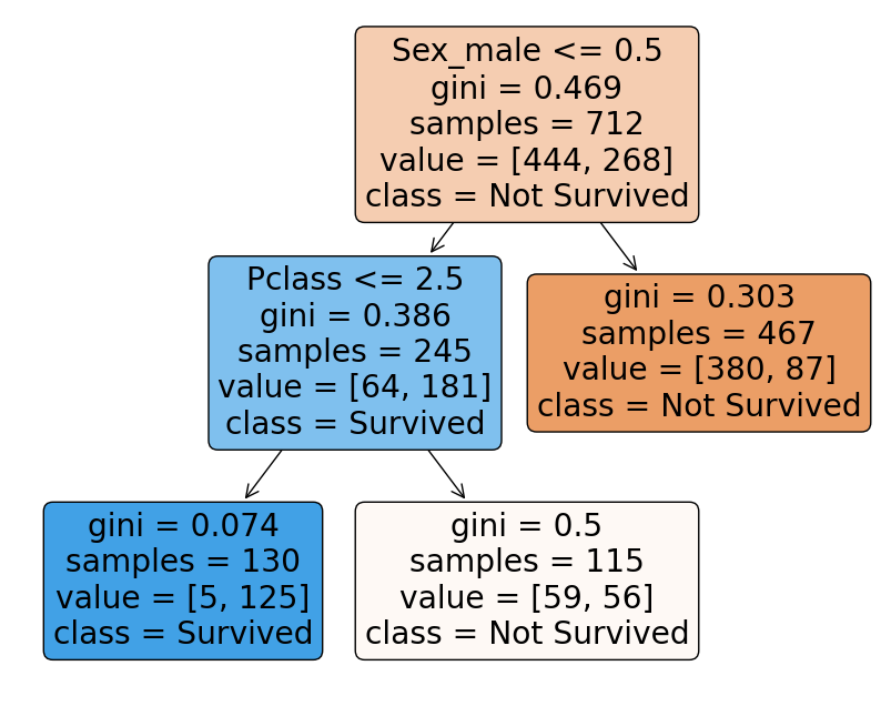
We can be aggressive and take $ccp_alpha = 0.015924$, as pruning does not significantly reduce the accuracy in this case. The result is the following Final pruned decision tree:

Conclusion

Lets compare the evaluation metrics for our our initial model and our interpretable model:

Metric	Best Mean	Final Mean	Best Std	Final Std
Accuracy	0.8103	0.7837	0.0121	0.0316
Precision	0.7966	0.8775	0.0185	0.1277
Recall	0.6812	0.5338	0.0559	0.1077
F1 Score	0.7325	0.6462	0.0302	0.0540
ROC AUC	0.8499	0.8039	0.0273	0.0357

We can see that the Final model provides comparable performance with much more interpretable decision tree.

Final Remarks

Here’s a more reader-friendly rewrite of your final remarks:

---

Final Remarks

When exploring topics like this, I prefer .py files over .ipynb notebooks, using IPython instead of Jupyter. I find this approach better aligns with production workflows while still offering the flexibility needed for exploration.

That said, presenting content in this format can be challenging. Reading through a full script isn’t always the most user-friendly experience, and you don’t need to wade through all the details. That’s why I took a different approach here. Instead of presenting a full Jupyter Notebook, I focused on the key steps of the workflow. With the help of the Data Archive, I’ve also provided an opportunity to dig deeper into related and tangent topics for those who are interested.

Thanks for reading! I hope this post helps you build more interpretable decision trees.