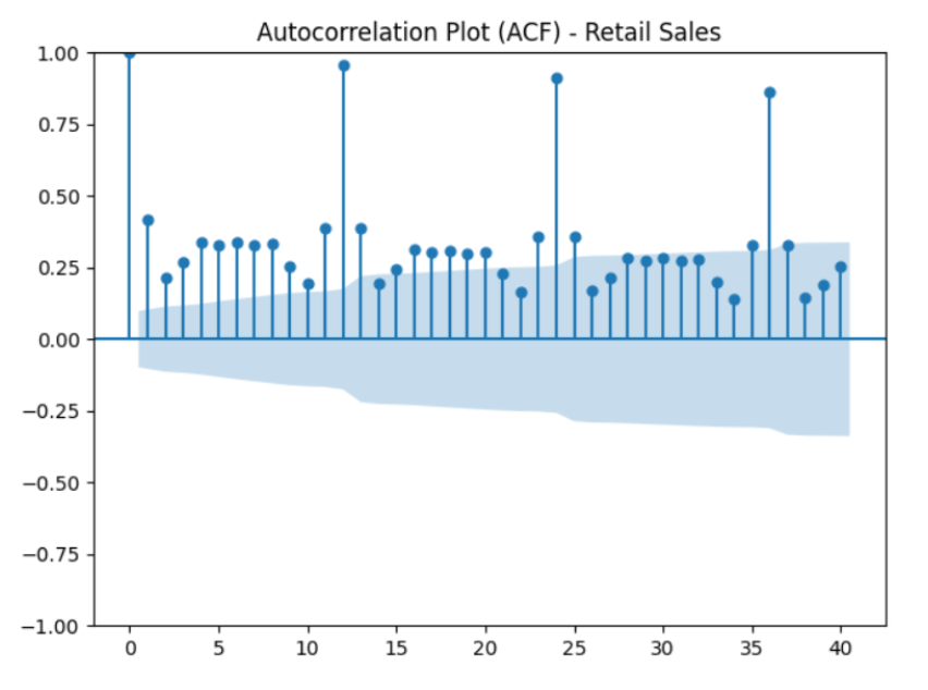
An Autocorrelation Function (ACF) plot shows how each observation in a time series is correlated with its past values at different lags (Forecasting using Lags). It helps identify trends, seasonality, and whether a series is stationary.
Understanding ACF Behavior
- In a Stationary Time Series, autocorrelations decay quickly toward zero as lag increases. This indicates past values have decreasing influence on future values.
- If autocorrelations remain high across multiple lags, this suggests:
- Trend: values persistently related over time (Trends in Time Series).
- Seasonality: repeating peaks at specific lag intervals (Seasonality in Time Series).
Key takeaway: Slow decay or repeated high correlations indicate a non-stationary series.
How to Interpret an ACF Plot
- Decay pattern:
- Rapid decay → stationary series.
- Slow decay → non-stationary series.
- Significant peaks: Regular spikes at certain lags indicate seasonality.
- Correlation magnitude: High correlations at large lags suggest trend or long-term dependencies.
Detailed Interpretation Guide
- Significant spikes outside confidence intervals → meaningful correlation at that lag.
- Gradual decay → indicates an autoregressive (AR) process.
- Sharp cutoff after a few lags → suggests a moving average (MA) process.
- Alternating signs → may indicate oscillatory behavior.
- Slow decay over many lags → possible non-stationarity or trend.
- Seasonal pattern → repeated peaks at multiples of seasonal lag (e.g., lag 12 for monthly data).
Additional Notes
- ACF includes indirect effects: e.g., correlation at lag 3 may result from correlations at lags 1 and 2.
- Apply ACF to stationary data; otherwise correlations may be misleading.
- Use ACF to determine in an MA() model.
Related
PACF Plots Forecasting with Autoregressive (AR) Models