PACF Plots

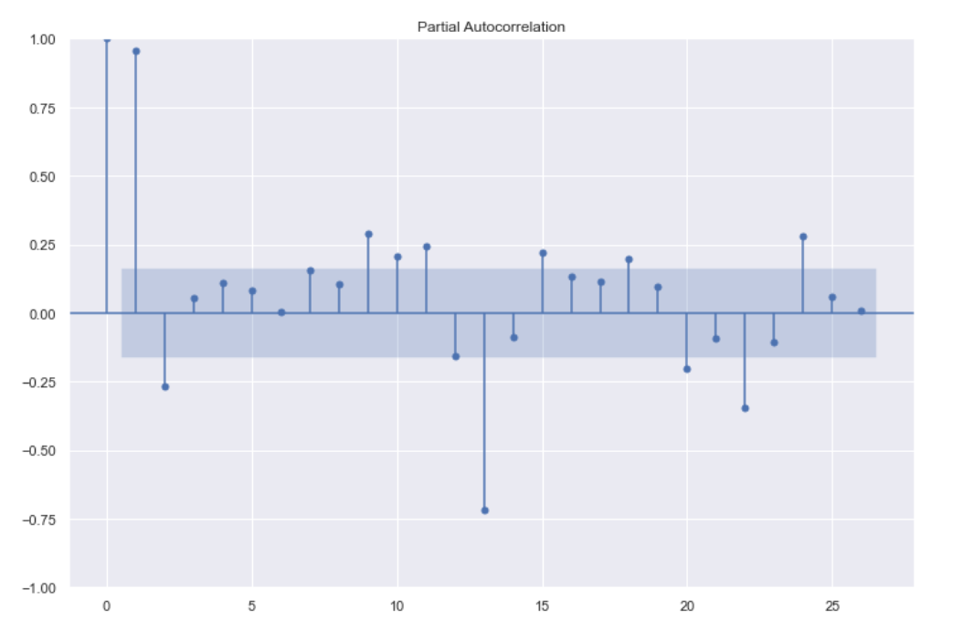
The Partial Autocorrelation Function (PACF) plot shows how a time series is correlated with its lagged values, ==while controlling for correlations at shorter lags.== For instance, in a series of air passengers, PACF reveals how much each observation is directly influenced by past values and identifies how far back statistically significant correlations exist.

PACF differs from the ACF Plots in that it isolates direct correlations, removing the effects of intermediate lags. Examining both ACF and PACF together provides a more complete view of the time series structure.

Purpose

The PACF is used to:

• Identify direct relationships between a time series and its lagged values.
• Determine the order $p$ for an autoregressive (AR) model.
• Complement the ACF in diagnosing stationarity, seasonality, and the underlying process type (AR, MA, ARMA).

How to Interpret a PACF Plot

• Significant spike at lag $k$ → indicates the direct influence of $X_{t-k}$ on $X_t$.
• Sharp cutoff after lag $p$ → suggests an AR($p$) process.
• Gradual decay → may reflect a moving average (MA) or mixed ARMA process.
• Few isolated spikes → implies only short-term dependencies.

Additional Notes

• The first significant lag in PACF often determines the AR order $p$.
• PACF complements ACF — together they guide model identification for ARIMA.
• If both ACF and PACF decay slowly, the series is likely non-stationary.

Decomposition in Time Series ACF Plots

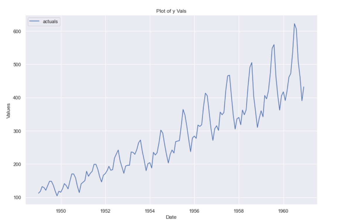
Dataset