Stationary Time Series

A stationary time series is one whose statistical properties do not change over time. Many classical time series models (e.g., ARIMA, SARIMA) assume stationarity. Non-stationary data can lead to misleading results expecially in Time Series Forecasting.

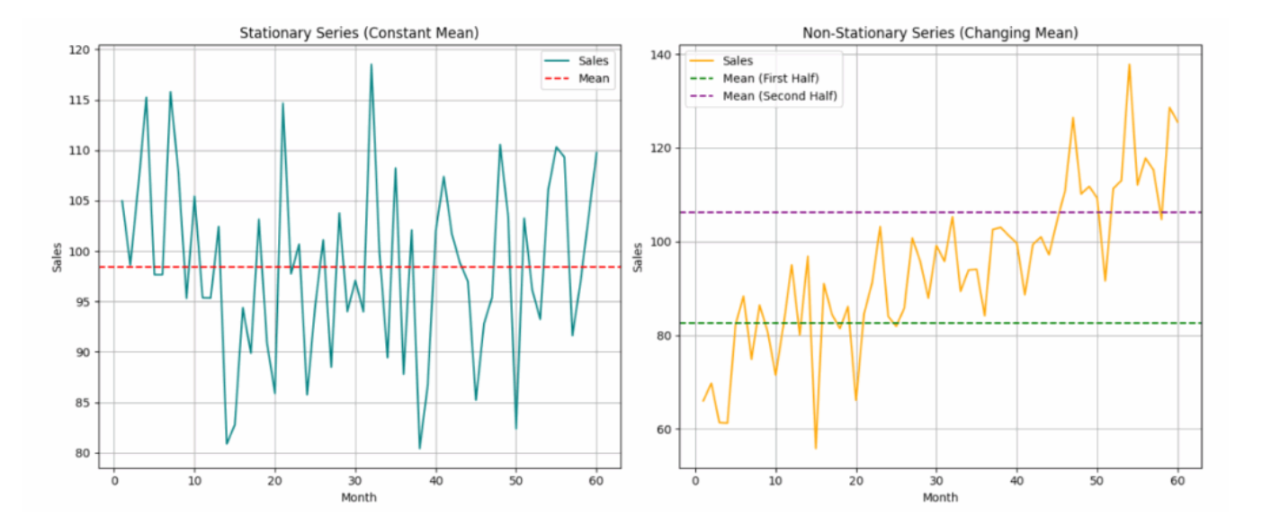
This means the process has the same behavior regardless of when you observe it. Checking a series’ stationarity is important because most time series methods do not model non-stationary data effectively. “Non-stationary” is a term that means the trend in the data is not mean-reverting - it continues steadily upwards or downwards throughout the series’ timespan.

Formally, a time series $y_t$ is stationary if:

• The mean is constant: $E[y_t]=\mu$ for all $t$.
  • 
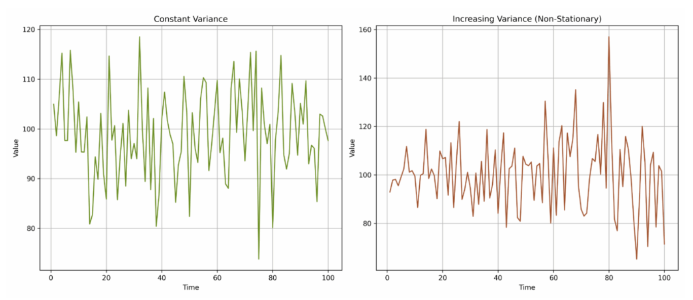
• The variance is constant: $\text{Var}(y_t)={\sigma }^2$ for all $t$ (the spread of data). If the time series goes up and down by similar amounts throughout the series, then it is said to have Constant Variance. More spread
  • 
• The autocovariance depends only on the lag $k$, not on the specific time $t$: $\text{Cov}(y_t,y_{t+k})={\gamma }_k$. If the relationship between values depends only on the gap between them, regardless of when they occur, then there is Constant Autocovariance.

Types of stationarity

1. Strict stationarity: The entire distribution of the process is invariant to shifts in time (all moments remain constant).
2. Weak (or covariance) stationarity: Only the first two moments (mean, variance, covariance) are invariant. This weaker definition is often sufficient for models like ARIMA.

Examples

Stationary: White noise (mean = 0, variance constant).

Non-stationary:

• Series with a trend (e.g., increasing sales over time).
• Series with changing variance (e.g., volatility clustering in finance).
• Series with seasonality (patterns repeating over time).

Trnasfomration to get Stationarity

Common Data Transformation to achieve stationarity include:

• Differencing in Time Series

• STL Decomposition
• Log transformation (to stabilize variance)
• Detrending or deseasonalising

Tests for Stationarity

Practical checks:

• An easy way to check for constant mean and variance is to chop up the data into separate chunks.
• Then, one calculates statistics for each chunk, and compare them.
• Large deviations in either the mean or the variance among chunks might indicate that the time series is nonstationary.

Statistical Tests:

• ADF Test & KPSS Test: Augmented Dickey-Fuller test give statistical justification to what our eyes see. If the the p-value is not less than 0.05, we must assume the series is non-stationary.
• Visual inspection with STL Decomposition
• ACF Plots

Related

• Decomposition in Time Series
• One time events (Interventions) be removed (think Covids impact of stock data). See Intervention Analysis.
• Decomposition in Time Series

Resources:

• https://towardsdatascience.com/time-series-forecasting-made-simple-part-4-1-understanding-stationarity-in-a-time-series/