In ML_Tools see:
Discrete Distributions
These distributions have probabilities concentrated on specific values.
- Uniform Distribution: All outcomes are equally likely. Example: Drawing a card from a shuffled deck. A boxplot can be meaningful if there’s variation in the distribution. Since the values are discrete, the boxplot will show the range and quartiles effectively.
- Bernoulli Distribution: Represents two possible outcomes. Example: Coin flip (heads or tails), true/false scenarios. A bar chart or frequency plot would be better for visualizing the proportions. or rolling a dice.
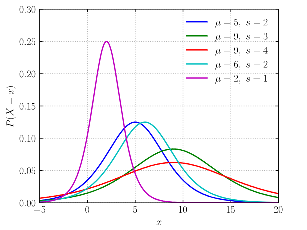
- Binomial Distribution: Represents the number of successes in a sequence of Bernoulli trials. Example: Number of heads in 10 coin flips,
- Poisson Distribution: Models the frequency of events in a fixed interval. Example: Number of website visits per hour. A boxplot is suitable for this distribution, showing central tendencies, spread, and potential outliers.
Continuous Distributions
These distributions have probabilities spread over a continuous range.
-
Gaussian Distribution: Characterized by a bell-shaped curve, symmetric with thin tails. Example: Heights, exam scores.
-
T Distribution: Similar to the normal distribution but with fatter tails, useful with limited data.
-
Chi-squared Distribution: Asymmetric and non-negative, commonly used in hypothesis testing.
-
Exponential Distribution: Models the time between events. Example: Time between website traffic hits, radioactive decay.
-
Logistic Distribution: S-shaped curve, often used in forecasting and modeling growth.
Practical Applications
Feature Distribution: Understanding the distribution of numerical/ categortical feature values across samples can provide insights into data characteristics.
- Observation: Analyze the spread and central tendency of data.
- Decision: Determine appropriate statistical methods or transformations.